In this project, we present a system for classification of musical instruments belonging to different instrument families exploiting the various temporal and spectral features that characterize the "timbre" of a particular instrument. Many features covering both spectral and temporal properties and their influences on a musical sound was investigated, and their extraction algorithms were designed.The features were extracted from the dataset that consisted of 558 samples covering the full pitch ranges of 10 orchestral instruments from the string, brass and woodwind families. The classification results consolidated the dependence of an instrument's timbral uniqueness on the features, especially the spectral ones. The correct instrument family was recognized with ~96 % accuracy and individual instruments within the families with over 95 % accuracy for each of the three families considered. Also, a hierarchical classification framework is utilized keeping the mind the taxonomic nature of musical sounds.
Link to Codes Used
1. Introduction
1.1 Introduction to Problem
Musical Instrument Identification by a computer has many scientific as well as practical applications such as automatic annotation of musical data, structured coding and ultimately developing a system that can understand music
enough to collaborate with a human in real-time performance.The goal of this project is to identify musical instruments from their audio samples using a statistical pattern-recognition technique.
1.2 Motivation
There are many scientific and practical applications in which musical instrument identification by a computer would be useful. Some of them are :
- Automatically annotating musical multimedia data
- Transcribing musical performances for purposes of teaching, theoretical study, or structured coding
- Ultimately, developing a system that can understand music enough to collaborate with a human in real-time performance
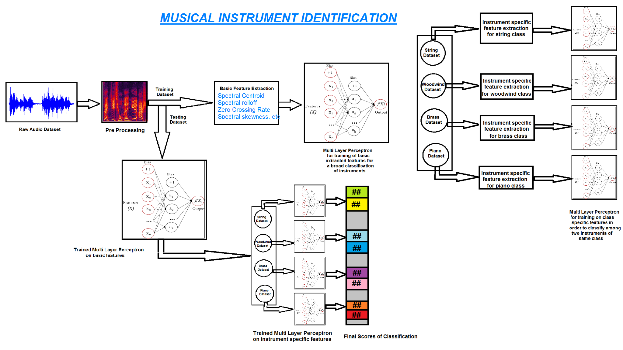
1.3 Figure
Block diagram of the Musical Instrument Identification approach
1.4 Literature Review
[1] Giulio Agostini,Maurizio Longari and Emanuele Pollastri,"Musical Instrument Timbres Classification with Spectral Features",EURASIP Journal on Applied Signal Processing 2003.
This paper addresses the problem of musical instrument classification from audio sources. A detailed analysis of spectral features and their precise description is presented along with their relative salience in the classification process. A number of classifying methods such as Discriminant Analysis techniques, Support Vector Machines and k-nearest neighbours have been tested and compared.
[2] Keith D. Martin and Youngmoo E. Kim, "Musical instrument identification: A pattern-recognition approach",Presented at the 136 th meeting of the Acoustical Society of America, October 13, 1998, MIT Media Lab Machine Listening Group Rm. E15-401, 20 Ames St., Cambridge, MA 02139.
This paper emphatically demonstrates that the acoustic properties studied in the literature as components of musical timbre are indeed useful features for musical instrument recognition. Starting from basic features, it follows a correlogram-based approach in classifying the instruments. Prominent features have also been discussed which influenced the classification process among the instruments belonging to a single family.
3] Antti Eronen and Anssi Klapuri, "Musical Instrument Recognition using Cepstral Coefficients and temporal features",Signal Processing Laboratory , Tampere University of Technology P.O.Box 553, FIN-33101 Tampere, FINLAND
In this paper, a system for pitch-independent musical instrument recognition is presented. A wide set of features covering both spectral and temporal properties of sounds was investigated, and their extraction algorithms were designed. Very high accuracy was attained with a certain set of features. Also, utilization of a hierarchical classification framework is considered.
[4] Antti Eronen,"Comparison of features for Musical Instrument Recognition",Signal Processing Laboratory, Tampere University of Technology P.O.Box 553, FIN-33 101 Tampere, Finland .
The paper intends to compare different features with regard to recognition performance in a musical instrument recognition system. The performance of earlier described features relating to the temporal development, modulation properties, brightness, and spectral synchronity of sounds is also analysed. The errors made by the recognition system are compared with the results reported by a human perception experiment.
1.5 Proposed Approach
Why do different musical instruments have different sounds?
Various characteristics of sound, such as loudness (related to energy) and pitch (related to frequency) determine how our brain perceives a musical instrument. BUT, if a clarinet and a piano play notes of the same pitch and loudness, the sounds will still be quite distinct to our ears. What , then , discriminates the sound of a clarinet from a violin ?
The answer is Timbre!
Timbre distinguishes different types of musical instruments, such as string instruments, wind instruments, and percussion instruments. It also enables listeners to distinguish different instruments in the same category (e.g. a clarinet and an oboe) .
Musical instruments do not vibrate at a single frequency: a given note involves vibrations at many different frequencies, often called harmonics, partials, or overtones. The relative pitch and loudness of these overtones along with other acoustic features give the note a characteristic sound we call the timbre of the instrument.
Timbre can be successfully used to distinguish between the 4 broad classes of musical instruments. After that we may use class-specific features to distinguish the instrument within the class.
Thus to achieve the goal of detecting the instrument being played in a given sound clip, we propose a two step approach:
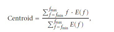
[1] In the first step we take advantage of the fact that musical instruments can be divided into 3 broad classes: Woodwind; String and Brass. Thus, we use a simple multilayer perceptron trained using basic timbre features : Spectral Centroid, Zero Crossing rate, Spectral Rolloff and Spectral Skewness among others. This helps to find the basic class to which the given musical instrument belongs and leaves us with the task of finding the exact instrument from within this basic class.
[2] In the second step, we train a classifer with individual class-specific features . This helps us to accuarately identify the musical intrument within the basic class as detected earlier.
Various characteristics of sound, such as loudness (related to energy) and pitch (related to frequency) determine how our brain perceives a musical instrument. BUT, if a clarinet and a piano play notes of the same pitch and loudness, the sounds will still be quite distinct to our ears. What , then , discriminates the sound of a clarinet from a violin ?
The answer is Timbre!
Timbre distinguishes different types of musical instruments, such as string instruments, wind instruments, and percussion instruments. It also enables listeners to distinguish different instruments in the same category (e.g. a clarinet and an oboe) .
Musical instruments do not vibrate at a single frequency: a given note involves vibrations at many different frequencies, often called harmonics, partials, or overtones. The relative pitch and loudness of these overtones along with other acoustic features give the note a characteristic sound we call the timbre of the instrument.
Timbre can be successfully used to distinguish between the 4 broad classes of musical instruments. After that we may use class-specific features to distinguish the instrument within the class.
Thus to achieve the goal of detecting the instrument being played in a given sound clip, we propose a two step approach:
[1] In the first step we take advantage of the fact that musical instruments can be divided into 3 broad classes: Woodwind; String and Brass. Thus, we use a simple multilayer perceptron trained using basic timbre features : Spectral Centroid, Zero Crossing rate, Spectral Rolloff and Spectral Skewness among others. This helps to find the basic class to which the given musical instrument belongs and leaves us with the task of finding the exact instrument from within this basic class.
[2] In the second step, we train a classifer with individual class-specific features . This helps us to accuarately identify the musical intrument within the basic class as detected earlier.
1.6 Report Organization
This project report is organized as follows.
[1] First, we give some background information on the importance of automatic Musical Instrument recognition and the motivation behind it.
[2] This is followed by the section on proposed approach where we discuss the approach towards the classification task. Some details about feature properties and their mathematical constructs are also presented.
[3] Then, a brief description of the dataset is followed by classification techniques employed in the project.
[4] Finally, results are presented along with the conclusion of the project. A short summary and possible future extensions close the report.
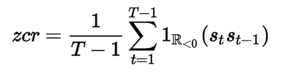 where s is a signal of length T and 1 is an indicator function.